Although I had planned to continue to work through the Discussion Topics from Bacterial Genetics and Genomics that are all related to the investigations in bacterial genetics and genomics using bioinformatics tools can be conducted outside of the lab, October here in the UK includes Biology Week. In addition to my research and teaching at the University, I also like to do outreach activities and public engagement in science, which includes going to schools to talk about biology, my career as a woman in science, and the cool things that we can do with genomics. One of the stories that the students and teachers find particularly fascinating is one that I was asked to deliver for Biology Week this year, but remotely, due to COVID-19. So, for this month’s blog, I have combined by regular blog with a video that I have produced for Biology Week about the outbreak of cholera in Haiti and how genomics helped to solve the mystery of its origin.
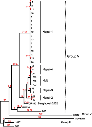
In January 2010, an earthquake struck Haiti causing widespread devastation. The international aid community responded, with the UN coordinating sending troops to help rebuild needed infrastructure and help the population. However, in October 2010, there was an outbreak of cholera that was traced back to the UN aid worker station and unsanitary conditions of waste disposal there. Ultimately, genome sequencing of the Vibro cholerae bacteria showed that it was nearly identical to bacteria from a recent outbreak in Nepal (doi: 10.1128/mBio.00157-11), as shown in the phylogenetic tree figure below. This genomic information links the outbreak to the arrival in October 2010 of UN aid workers from Nepal. Although none of these people who had come to help had symptoms, this emphasizes the role that asymptomatic carriage has in the spread of infections during an outbreak.
Phylogenetic tree showing cholera bacteria from Haiti are nearly identical to cholera from Nepal. Hendriksen et al., mBio, 2011.
Using metagenomics, the sequencing of environmental samples of DNA, researchers investigated the prevalence of cholera in Haiti in the years following the initial outbreak. Monika A. Roy and co-authors published in 2018 their metagenomic approach to evaluating surface water quality in Haiti (doi: 10.3390/ijerph15102211). In their publication, they note that since the earthquake in January 2010 and the subsequent cholera outbreak in October 2010, there had been over 9,000 deaths from cholera in Haiti.
During the term of their investigation, cholera cases had declined, but were still occurring and one of the issues was the inability to predict where new cases might occur due to gaps in surveillance. Through use of metagenomics to monitor groundwater it was hoped this might identify sources of potential cholera contamination.
The cost of using genomics for metagenomics monitoring of environmental samples is mentioned in the Introduction of the paper by Roy et al., 2018. They mention the availability of handheld MinION devices, such as those discussed in my previous blog entry, but cite that the regents to run one flowcell cost $1000. They concede that if samples are multiplexed, mixed together with molecular barcodes to differentiate them so more samples can be run at once, then the per sample cost can be reduced to $80 per sample.
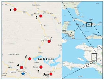
Water samples were collected in 2017 as a pilot investigation and then again from specific locations in triplicate in 2018. The water was filtered using 0.22 μm filters. This is the same size filter we would use in the lab to make solutions that cannot be autoclaved, but which we need to be sterile. Therefore, bacteria in the water would be trapped onto the filters and the DNA from these was later extracted in the lab using a QIAGEN kit. This DNA is a mixture of DNA from the environment, thus being a metagenomic sample, which was sequenced using an Ion Torrent sequencer. The data was processed using CosmosID to gain the results that were interpreted by the team.
Map of regions of Haiti where water samples were taken for metagenomic sequencing. Roy et al., Int J Environ Res Public Health, 2018.
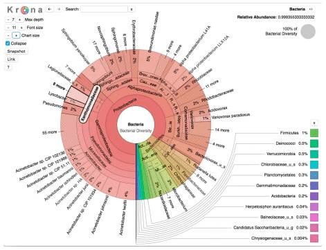
Another issue is the bioinformatics, but again the authors acknowledge that there are improvements here in making workflows easier to use and better optimized. Using the popular Krona visualization tool for metagenomics analysis, the diversity of organisms revealed is presented. They noted that V. cholerae was present in most of the replicates of water samples, although at varying abundance. The researchers are careful in their experimental design and note that V. cholerae is not always pathogenic; this is also an environmental bacterial species and when investigating metagenomics, markers must be selected to identify pathogenic versus non-toxigenic strains. The Haitian strain HE-45 was detected and samples with the virulence gene V. cholerae intI1 were identified. Cholera toxin converting phage was detected in one sample from a source not known to be used as drinking water, however these places are used for bathing, washing clothes, and for other household activities that could result in accidental ingestion of contaminated water. In addition to the cholera toxin gene, sequences for Shiga toxin were also detected. A distinct advantage of a metagenomics approach is the identification of sequences that were perhaps not part of an original hypothesis; if the initial concern had been about cholera and the investigation had just looked for cholera, these other sequences of concern would have been missed. Shiga toxin is made by EHEC E. coli such as O157:H7 and can cause life threatening disease.
Krona visualization of Haiti water source metagenomic data showing diversity of organisms present. Roy et al., Int J Environ Res Public Health, 2018.
The conclusion of the metagenomics study was that no V. cholera O1 or O139 strains were detected, which was consistent with the decline in cholera cases, however the presence of cholera toxin genes and Shiga toxin genes in the water was concerning. These could indicate potential risks for the populations using this water.
The last case of cholera in Haiti was seen in January 2019. Control of the outbreak has taken a tremendous effort in re-establishing clean water and sanitation that was destroyed by the hurricane and improving upon the infrastructures of Haiti, as well as implementing other control measures such as vaccination and rapid tracing and treating systems. In April 2019, there were concerns that the apparent eradication of cholera in Haiti should not be taken as a sign that the nation could cease being vigilant. High standards in potable water, sanitation, and healthcare must still be emphasized as of fundamental importance for preventing outbreaks across the globe.
The publications of the first bacterial genome sequences were 25 years ago. The technology has come a long way since then, both in the lab and computationally. One of the first bacterial genome sequencing projects started was one undertaken to sequence the complete Escherichia coli genome. Ultimately, it was completed and published in 1997. To-date, this publication has been cited by 2,469 other articles, including a recent investigation into E. coli that are present on the surface of the human eye (Ranjith et al., 2020).
E. coli are predominantly found in the intestinal tract of humans and animals, but they are also present elsewhere, including on the ocular surface. There are, in fact, many bacterial species that reside as commensal, non-pathogenic, bacteria on the surface of the eye. These bacteria can cause opportunistic ocular infections when there has been trauma to the eye or due to other issues that compromise the immune system. To understand more about this type of E. coli, 10 eye isolates were genome sequenced. The genome sequences were analyzed for SNP variation to find single nucleotide polymorphisms between the sequences. The isolates were sorted into the nearest E. coli phylogenetic group and pathotype, as well as being assessed for antimicrobial resistance genes, prophages, and other factors that might be involved in pathogenicity.
The E. coli isolates came from two cases of conjunctivitis, two cases of bacterial keratitis, five cases of endophthalmitis, and one from orbital cellulitis. DNA was extracted from overnight cultures of the E. coli using a QIAGEN DNA isolation kit and genome sequenced using an Illumina HiSeq. The data was mapped against the reference genome sequence E. coli strain K-12 substrain MG1655 using BWA. The de novo assemblies used Velvet.
From this study, antimicrobial resistance genes were identified, which correlated with antimicrobial investigations in the laboratory. Five out of the 10 isolates were resistant to more than three classes of antibiotics. Presence of plasmids, prophages, and virulence genes were also identified, including some that may be characteristic of ocular isolates.
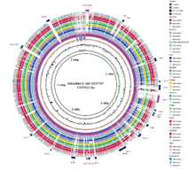
The different presence and absence of virulence genes, resistance genes, prophages, and plasmids were examined using BRIG, the BLAST Ring Image Generator, an example of which is described in Chapter 17 of Bacterial Genetics and Genomics and shown in Chapter 17 Figure 12 (shown below).
BRIG, BLAST Ring Image Generator, example image from Bacterial Genetics and Genomics, Chapter 17, Figure 12. Comparative visualization of E. coli genome sequences.
The 10 isolates were also able to be categorized into three of the seven known phylogenetic groups: A (2 isolates); B2 (7 isolates): and C (1 isolate). SNP analysis agreed with these relationships. Additional analysis associated the ocular isolates with four of the eight pathotypes, grouping six isolates with ExPEC (extra-intenstinal pathogenic E. coli), two with EPEC (enteropathogenic E. coli), on wit ETEC (enterotoxigenic E. coli), and one with UPEC (uropathogenic E. coli)strains. There was therefore a lack of concordance between the phylogenetic groups (A, B2, and C) and the pathotypes (ExPEC, EPEC, ETEC, and UPEC).
This study, and the over 2,000 others that have cited the original E. coli genome sequence paper, as well as many others, have shown the power of genome sequence data in revealing both differences and similarities between bacterial strains. There is tremendous diversity in the microbial world. The more we sequence, the more that is apparent. We have come a long way in 25 years. Not only are many genome sequence papers published currently that include more than one genome, but such studies are able to comparatively analyze the data, identify features that we did not know were present when investigations first started, generate the data and analyze it in a fraction of the time, and do so using much less starting material than previously required, including generating sequence data without first culturing bacteria in the lab.
For this blog, I have decided to look at the Discussion Topic from Bacterial Genetics and Genomics, Chapter 16, question 15, which discusses restriction enzymes and encourages us to try finding digest sites for these enzymes ourselves in a gene of interest, using on-line tools. In the spirit of the last few blogs (see Doing research and making discoveries outside of the lab and More research outside of the lab, protein structure predictions), since many of us are working at home during the pandemic, either exclusively or with limited access to our labs, I have decided to take an approach that uses a minimum of tools to achieve the final goal. This means that regardless of your set up on your computer, you should be able to complete the task of identifying two restriction enzyme recognition sites, the places where the enzyme would digest the DNA. We want enzymes that would generate sticky ends and that will cut only once in the gene sequence, with one enzyme cutting at the beginning and one at the end of our gene of interest.
I’m going to use the same hypothetical gene that I investigated in the previous blogs. So far, I have been using the predicted protein sequence. This is easily extracted out of an annotation. Annotation files are plain text files and can be opened with a text editor file. I recommend Notepad for those using Windows because Notepad doesn’t add any formatting; a word processing programme like Word does add formatting, even to plain text files, so keep it simple with something like Notepad that opens .txt type files when you want to open FASTA and annotation files such as those downloaded from GenBank. Google tells me that Mac users can use TextEdit, but you need to be sure the format is plain text. I’m not a Mac person, so I don’t know for sure, but maybe someone can verify in the comments.
Since the annotation will list the amino acid sequence as part of the annotation, it is simple to copy and paste out the predicted protein sequence. The sequence of the annotated coding region, the CDS, which is the prediction for what might be a gene, is indicated by the base locations. The actual sequence of the CDS is part of the DNA sequence information as a whole. So, to get the specific sequence of CDS or a specific gene, we need to extract it out.
If we are working in a public database like NCBI GenBank, we can retrieve the sequence data or restrict it to just show the specific base range we need for the CDS. However, I am working with my own sequence information, which I have as the plain text, flat file of the annotation, in GenBank format. I could use a specialist program to open it and extract out the DNA sequence for the gene I need. But, I don’t have to do that. And, the purpose of this blog is to show you that you don’t need that and it can be done on any computer, with a bit of internet and some copying and pasting. No special software required.
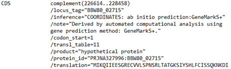
In my case, I already know what sequence I want. I know from the annotation that it is present at “complement (226614..228458)”.
Screenshot of a portion of a GenBank format annotation of sequence for a CDS designated as a hypothetical protein.
Interesting. The designation “complement” and the numbers in parentheses mean that the sequence of this predicted gene is going to be in the DNA in reverse complement. That means that the 226614 is going to be the end of the CDS and the 228458 is going to be the beginning. This is not what we might have expected, so something to watch out for when working with DNA sequences. Remember, the genes can be on either strand of the double helix. If the CDS was on the forward strand it would have just had the numbers to the right of the designation CDS without “complement” and the “()”.
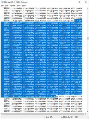
I scroll through my file in Notepad and find the DNA and then the location of the CDS. It is possible then to highlight the CDS and copy the needed DNA sequence. Yes, this is the very low tech solution for doing this. There are other ways and programs that will achieve the same thing for you, but I wanted to show what can be done, by virtue of sequence files being plain text and therefore easy to manipulate on any computer.
Note that the first bases highlighted are TCA, which in reverse complement are TGA, a termination codon or stop codon. The last three bases are CAT, which would be the ATG reverse complemented initiation codon of the CDS. This is a good way to double check that you have the right area highlighted; check that you start and stop with an initiation and termination codon and that these are on the strand you expected based on the annotation.
Screenshot of a portion of a GenBank format of sequence data showing the DNA, with a portion highlighted in blue representing the CDS under investigation.
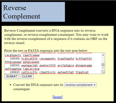
If this was on the forward strand, I could paste it straight into a new Notepad file and make it a FASTA file of my own. But, it is in reverse complement, so I need to fix that first. There is a handy site to do this, which has not changed in many years: https://www.bioinformatics.org/sms/rev_comp.html. This does the basic operation needed.
Screenshot of the web interface for Reverse Complement on-line program to covert DNA to its reverse complement. Shown is a window to paste in the sequence of interest, a button to Submit for conversion, and a button to Clear the entry.
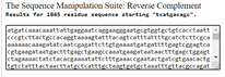
All of the non-DNA characters (the numbers from the annotated file) are deleted during the process. This is good. The output is the DNA in the right orientation, from the ATG start to the TGA stop.
Screenshot of the output from Reverse Complement on-line DNA conversion.
The sequence is copied out of the Sequence Manipulation Suite output into a new Notepad file and made into a FASTA file through my addition of a line at the top that starts:
>Blog CDS for restriction digestion
Now that I am all set with the sequence of a gene – or in this case a sequence that has been predicted to be a gene – I can see which restriction enzymes might cut it.
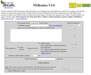
The recommendation from Chapter 16 is to try NEBcutter:
Screenshot of NEBCutter v2.0 on-line web-based interface. Input options include selecting a file, accession number, or pasting a sequence into the space provided, before submitting the sequence to identify restriction enzyme cut sites.
I paste my sequence into the box to see which NEB enzymes will cut and get this output:
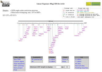
Screenshot of the NEBCutter output for the gene of interest, showing a graphical representation of the locations of restriction enzyme cut sites along the length of the sequence. There are links for other options at the bottom of the page.
So, that’s the first part of Discussion topic 16.15 done. I have identified the enzymes that would cut the sequence. This on-line tool gives me a graphical output of the length of the CDS and shows where along it the various enzymes would cut. There’s more investigation that can be done from here, including zooming in and refining what is shown.
The Discussion topic wants me to identify those restriction enzymes that cut the CDS only once. This is easily done here on the NEBcutter tool. There is a link under the List heading that says “1 cutters”. I press that and all of the single cutters are listed, either alphabetically or by cut position.
The next parameters that the Discussion topic wants me to explore is to find:
One enzyme that cuts at the start of the gene and generates sticky ends
One enzyme that cuts at the end of the gene and generates sticky ends
Both of the identified enzymes need to work at the same temperature
Both of the identified enzymes need to work in the same buffer
To achieve the end goal I will change the sort order from alphabetical to cut position. Looking through the information on the first few, I am going to look first at XbaI. Why? This is an enzyme that I recognize and I think we have some in the freezer, so that will save on time and cost to use something we already have. I could pick anything and order something new, but I might as well use an enzyme from the freezer if it works for the experiment. Here the XbaI cuts T CTAGC with a 5’ overhang at 37°C in CutSmart Buffer at position 232/236.
Now I need one at the other end. There I find HindIII catches my eye, again as something we likely have in the freezer. It cuts A AGCTT with a 5’ overhang at 37°C in NEBuffer2.1 at position 1580/1584. That doesn’t look great, being in a different buffer from XbaI and at first I think I might need to look for a different enzyme on the list. However, there is more information on each enzyme on the product list page and I’ve just been looking at a summary.
Delving deeper, I see that HindIII has 100% activity in NEBuffer 2.1, but only 50% in CutSmart Buffer, so no help there. However, checking the product page for XbaI, I find out that it has 100% activity in CutSmart Buffer, but it also works at 100% in NEBuffer 2.1. So in NEBuffer 2.1 at 37°C I can do a double digest of the CDS under investigation with XbaI and HindIII, which will generate incompatible sticky ends and delete out 1348 bases of the coding region. I could then also digest an antibiotic resistance cassette marker with XbaI and HindIII to join with the cut ends and make selection of deletion mutants possible. Homologous recombination between the flanking regions brings the resistance marker into the chromosome, deleting the gene in the process, and the bacterial cells that are resistant to the antibiotic are those that have the gene deleted.
All of the digestion, ligation, and generation of the mutants would, of course, happen in a lab, but the planning of the experiments, such as investigating the presence of the restriction digest sites, can be done outside of the lab. Good planning of experiments is essential to making sure that experiments work well. Take the time now to plan experiments carefully. Think through protocols, write them out, and ensure they are really robustly planned, so that when you do go into the lab you have done everything you can to ensure success.
Figure extracted from Bacterial Genetics and Genomics showing insertion of a resistance marker into a gene of interest to generate a construct, which is then transferred into the chromosome to generate a knockout mutant.
There are several other ways to achieve knock-outs and generate other mutations that are described in Bacterial Genetics and Genomics, as well as other uses for restriction enzymes. There are also great resources available on-line to support your use of the book, including slides with the figures from the book, like the one above, and flashcards to assist with learning terms.
That’s it for my blogs for Chapter 16, Gene Analysis Techniques. Next month I will get started on Chapter 17, Genome Analysis Techniques in my continuing theme on supporting research outside of the lab.
Continuing on from the blog post last month, I am keeping on the topic of research that can be done at home, or at the computer, without needing to do experiments in the lab. Quite a lot of genetics and genomics research today involves the investigation of data and analysis of that data using computational approaches. This requires a lot of care, time, and attention at the computer, so there is plenty that can be done outside of the lab to advance our research.
This week, I have drawn from the Discussion Topic question at the end of Chapter 16 in Bacterial Genetics and Genomics. This chapter focuses on gene analysis techniques. This second Discussion Topic asks us to look at what we can learn about the structure of a bacterial protein from just its amino acid sequence.
As we know from the rest of the book, the amino acid sequence itself is based on the codons encoded in the DNA sequence. These form the string of amino acids that we can read on a page, but this is not how the amino acids are present in the protein. Those amino acids, joined together by peptide bonds, are folded and twisted in upon each other, to form a three-dimensional structure, maybe on its own, maybe with other copies of the same protein, or maybe with other proteins.
Using the same amino acid sequence that I used in last month’s blog, I am going to see if I can find a structure to the hypothetical protein that I investigated. Since it is hypothetical, it is highly unlikely that anyone has crystalized and experimentally determined the structure of this specific protein; it is not likely to have been previously investigated, since the function hasn’t been determined. But, there may be another protein that is similar to it for which a structure is known.
As for last month, I have the protein sequence in FastA format, which has a first like starting with “>” followed by some information about the sequence, and then the sequence data starting on the second line:
>Hypothetical protein for blog post analysis
MIKQIIEE….
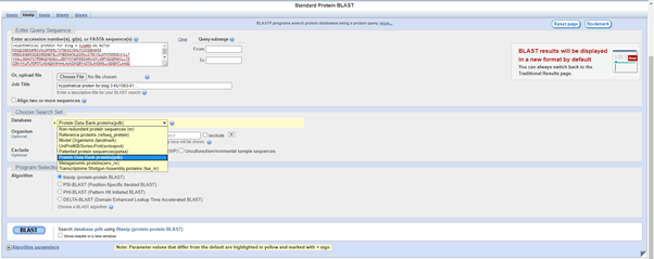
One strategy is to do a BLASTP search. You may be thinking – but Dr. Snyder, you did that last month. Yes, I did, but this time, I will alter the settings somewhat.
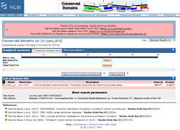
On the BlastP screen, I have pasted my FastA format sequence into the query field. In the Choose Search Set, rather than searching the Non-redundant protein sequences (nr) as I did last month, today I am searching the Protein Data Bank proteins (pdb). This is a repository of 3D protein structures and other large biological molecules.
Screenshot image of BlastP landing page. Hypothetical protein sequence has been entered as the Query Sequence and Protein Data Bank has been chosen as the Search Set from a pull down menu.
When I press BLAST, I get this result. Not great, since there is only one hit and it is to an algae Euglena gracilis.
BlastP result from the previous image, showing one hit to the Query sequence: Chain G, subunit b from Euglena gracilis.
The E value is terrible at 9.3. The query coverage is only 7%, as is graphically evident in the graphic summary tab:
BlastP search results showing the Graphic Summary. This displays the E. gracilis hit region of similarity against the length of the Query. There is a very short black bar visible near 400 where the sequences align.
The small black bar under the 400 position is the area where there is some similarity between my hypothetical protein and the E. gracilis protein hit. This is the alignment, which shows just how few amino acids align between the two proteins.
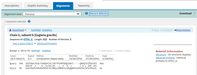
BlastP search results showing the Alignment between the E. gracilis hit and the Query. A short region of the Query is shown from 396 to 444 amino acids that have some similarity to the E. gracilis protein sequence (35% identity, 19/54).
There might possibly be enough similarity in this region to suspect that the structure of this part of the protein, maybe the folds involved there, might be similar, but I’d be much happier if I had come across the structure of something with some much closer similarly.
However, for the purposes of illustration in the blog, let’s have a look. Returning to the Descriptions tab, there is information about the E. gracilis hit, including the Accession number 6TDV_G.
BlastP results shown previously with the one E. gracilis hit. Data for the hit includes Max. Score 28.9, Total Score 28.9, Query Cover 7%, E value 9.3, Per. Ident 35.19%, and Accession 6TDV_G.
Clicking on this link takes me to the entry for this sequence and structure data.
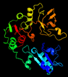
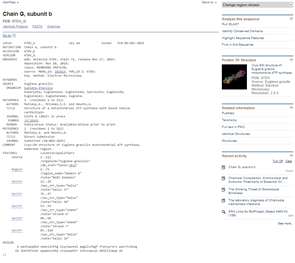
Accession 6TDV_G entry for E. gracilis Chain G, subunit b protein. The GenPept format entry is shown to the left and an image of a 3-dimensional protein structure is in the right margin under the heading Protein 3D Structure.
Clicking on the Protein 3D Structure picture at the right brings me to the 3D model, which is available in formats that mean I can set it to spin and show the full 3D rotation display in a full-featured 3D viewer.
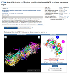
Cryo-EM structure of E. gracilis mitochondrial ATP synthase, membrane region. Page for Accession 6TDV_G includes a detailed description of the whole protein of 29 subunits and shows the 3D protein structure.
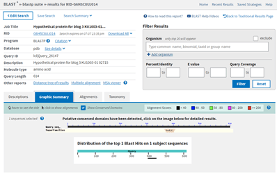
Since there is so little similarity and since what little similarity there is matches a small portion of this larger structure, I am going to leave that bit of analysis and try something else. You might have noticed from the BlastP results that on the Graphic Summary tab there was some additional information. Note where it says: Putative conserved domains have been detected, click on the image below for detailed results. This is generated because when a BlastP is run, it also runs a Conserved Domain search (https://www.ncbi.nlm.nih.gov/Structure/cdd/wrpsb.cgi). This result is not always present; it only shows up when the Conserved Domain search finds a conserved domain in the query protein sequence.
BlastP result Graphic Summary display, as previously. Above the previously noted graphic showing where in the Query protein the hit aligns, is the graphic indicating there have been Conserved Domains detected.
Clicking on the image for the conserved domains, I can see that there is a UvrD-like helicase C-terminal domain.
Conserved Domain search results. Listed are the protein domains identified, here UvrD_C_2 and a short description “UvrD-like helicase C-terminal domain. This domain is found at the C-terminus of a wide variety…”. Descriptions are expanded by pressing the {+} to the left of the name.
To learn more, I click on the [+] next to the name of the domain. The additional information tells me that this domain is found at the C-terminus of a wide variety of helicase enzymes and that the domain has an AAA-like structural fold. This may fit with some of the PSI-BLAST results from last month, which hit on some AAA family ATPases, and should be investigated further to find out about these types of proteins and the importance of this domain and its structure.
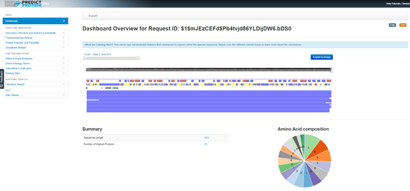
Out of curiosity, to see if any additional information can be yielded about the protein from other sources, I tried the PredictProtein search (open.predictprotein.org). This web-based search includes “whatever can reasonably be predicted from protein sequence with respect to the annotation of protein structure and function.” Because it does so many analyses, this took a while, but there were some results that came from it.
ProteinProtect results for the query hypothetical protein. There are several layers of graphical output displayed horizontally, followed by a summary that indicates the Sequence Length is 614 and the Number of Aligned Proteins is 31. A pie chart displays the Amino Acid composition.
In the blue message bar at the top it says, “What am I seeing Here? This viewer lays out predicted features that correspond to regions within the queried sequence. Mouse over the different coloured boxes to learn more about the annotations.” Doing that across the boxes above the solid blue lines, where there is a row of red and blue boxes, I find that the red boxes indicate potential helices and blue boxes are potential strands. So, that gives us some structural information already, which will be based on the potential of the amino acid sequence and the properties of the side chains of those amino acids. The next line down has yellow and blue boxes. The blue boxes here are regions of the protein that are predicted to be ‘exposed’ as in they are surface exposed on the 3D protein, while the yellow boxes are those that are ‘buried’ within the protein once it is folded. It is interesting to compare the data from the first line with the second here.
There is a lot to explore here. Clicking on the link Secondary Structure and Solvent Accessibility in the menu on the left shows that information in more detail.
PredictProtein result for Secondary Structure and Solvent Availability. This focuses on some of the data shown in the previous image, where red and blue blocks in one row show predicted helices and strands and the next row’s yellow and blue blocks show predicted exposed and buried regions. Pie charts are here for these features. On the left is Secondary Structure Composition with strand, helix, and loop wedges. On the right is Solvent Accessibility with exposed, buried, and intermed.
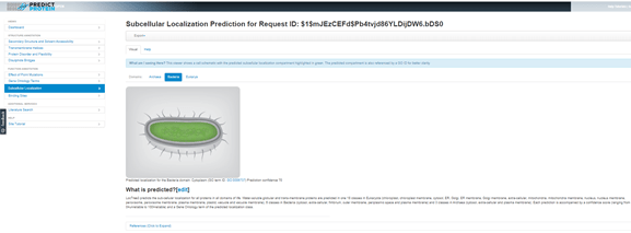
Clicking on Subcellular Locations from the left menu gives a prediction of where the protein might be located in the cell. I need to select the Bacteria tab here, because the default assumption is Eukarya, but the analysis has been done and the results are there waiting for me. Since the results so far suggest that this hypothetical protein might have enzymatic activity, it is not surprising that the location prediction is ‘cytoplasm’.
PredictProtein results for Subcellular Location. The Bacteria tab has been selected. A graphic of a rod-shaped bacterial cell is shown. Below this is written, “Predicted localization for the Bacteria domain: Cytoplasm (GO term ID: GO:0005737) Prediction confidence 70
In each case where a prediction is made the evidence is presented and there are references cited at the bottom of the page for the tools used to generate the predictions, so that both the PredictProtein and original tools references can be cited in any publications that might result from research using this web resource.
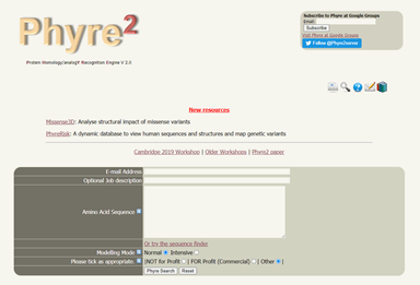
There are a variety of additional tools that can be used on protein sequences to analyse them and perhaps understand something more about the sequence. To see if perhaps I can understand any more about the possible structure of this protein, I decided to try Phyre2 (www.sbg.bio.ic.ac.uk/phyre2), Protein Homology/analogY Recognition Engine V 2.0. This uses remote homology detection methods combined with analysis of the primary amino acid sequence data to construct a 3D protein structure.
Home page for Phyre2 where users can enter their e-mail address, optional job description, amino acid sequence, modeling mode (normal or intensive), and tick as appropriate being ‘not for profit’, ‘for profit (commercial)’, or ‘other’. There is a Search button and Reset button.
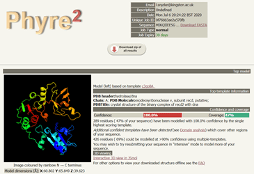
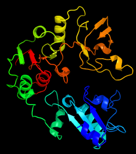
Again the results took some time to generate. Remember, these are computationally intense processes being done at PredictProtein and Phyre2, so be patient. In fact, Phyre2 gives users the option of running the modelling in Normal or Intensive Mode. I chose Normal for the sake of time, but for research, I would likely got back and do Intensive. In the end it was worth waiting for the results, because I got a lovely image of a potential protein structure to associate with my hypothetical protein of interest. It can be viewed in 3D mode as well, so I can move it around with my mouse and have a look at the structure from all angles.
Phyre2 results from hypothetical protein query. A protein structure is shown on the left. On the right is information for the top model: Model (left) based on template c3gp8A. Top template information is also displayed, including: PDB header: hydrolase/dna and Confidence 100% and Coverage 47%. There is a link for Interactive 3D view in JSmol.
More models are presented farther down the page in a table, displayed in order of decreasing confidence scores. Beside each is a graphic indicating the portion of the input protein sequence that has been represented by the model.
Phyre2 results displaying additional models in a table.. Column 1 numbers the models, column 2 gives the Template for the model, column 3 is a graphic of the Alignment Coverage, column 4 is images of 3D models, column 5 is Confidence as a percentage, column 6 is the percent i.d., and column 7 has template information.
All of the results I have been looking at in this blog are predictions. The protein, when made in the bacterial cell, may fold very differently from these predictions and it should be remembered that biologically protein structures can and do change due to a variety of factors like temperature, substrate binding, and phosphorylation. However, prediction can be used as a guide for experiments and investigations. If, for example, I was investigating a gene containing a SNP, which changed an amino acid in the encoded protein, I might want to know where that amino acid was located in the final protein structure. Predictions like these might help identify the location of the changed amino acid. Is it embedded inside a membrane? Is it buried within the folded protein? Or is it prominently on the surface of the protein where it might be important for interacting with other proteins or within what is believed to be the active site of an enzyme where it is involved in the binding of substrate?
I hope that this blog and the one before has been useful in demonstrating some of the tools available for doing research outside of the lab. This theme will continue next month when I tackle the last discussion topic of Chapter 16 and investigate restriction enzyme digest sites.
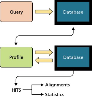
Graphical representation of PSI-BLAST, the tool used in this blog as an example.
At the time of writing this blog many of us find ourselves at home due to the COVID-19 pandemic. This has necessitated a change in focus for our research; for many of us our research laboratories are closed and we are working from home, socially isolating in an effort to reduce transmission of the virus.
Investigations in bacterial genetics and genomics using bioinformatics tools can be conducted outside of the lab. This means that so long as you have an internet connection, you can do meaningful research and make meaningful discoveries. In Chapter 16 of Bacterial Genetics and Genomics, some of the tools that can be used to explore bacterial genes are introduced. At the end of this Chapter, Gene Analysis, the three Discussion Topics suggest some ways in which these tools can be explored. In this blog and the next few that follow, I will work through these three Discussion Topics as examples of some of the things that we can do at home and at our computers to do research and make discoveries outside of the lab.
First tool we are going to explore using is PSI-BLAST. This is one of the suite of BLAST tools, which enable us to search for DNA or protein sequences that are similar to our sequence of interest. This can tell us if there are other sequences similar to our sequence in the public databases, which might tell us something about the sequence. Unlike the other BLAST searches, PSI-BLAST looks for more distant relationships between sequences by searching for similar sequences and then using those similar sequences to search again and again. This can be useful when trying to track down protein sequences that are distantly related or when trying to find a function for a hypothetical protein that otherwise is only similar to other hypothetical proteins. Hypothetical proteins are how we designate the potential products from regions of DNA that look like they could possibly be genes, but which don’t share similarity to known proteins. Hypothetically, the stretch of DNA may be a gene that encodes a protein, but it doesn’t look like anything else other than perhaps other hypothetical proteins.
I am starting with a hypothetical protein sequence from some genome sequence data we are investigating in my research group. To keep track of the protein sequence, I have pasted it into a Notepad file and saved it in FastA format. I’m using Notepad because this means that there isn’t any extra formatting added to the file that might interfere with any of the analysis that I want to do. When I save the file it will just be saved as plain text. To make it FastA format, I add a line at the top that starts with the greater than symbol “>” followed by any identifying information I’d like. So my file look something like this at the beginning:
>Hypothetical protein for blog post analysis
MIKQIIEE….
I haven’t included all of the protein sequence here, but in total my protein is 614 amino acids.
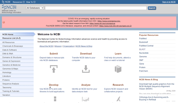
Now that I have the sequence all I need to do is run it through PSI-BLAST. To do this I go to the NCBI website http://ncbi.nlm.nih.gov
Image of the NCBI main page.
At the right hand side of the page, under Popular Resources, is a link to BLAST. I follow this link to the BLAST page http://blast.ncbi.nlm.nih.gov/Blast.cgi
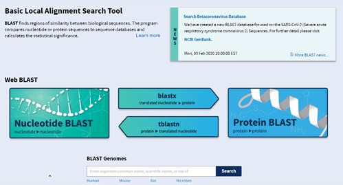
Image of the NCBI Basic Local Alignment Search Tool page.
PSI-BLAST is a Protein BLAST, so the next click is on the blue box that says Protein BLAST, with the graphic of the protein alpha helix structure on it. This takes us to the BLAST suite page.
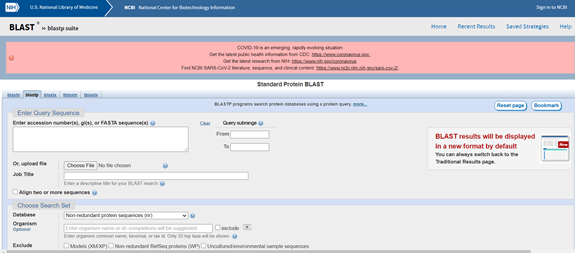
Image of the Standard Protein BLAST submission form (top).
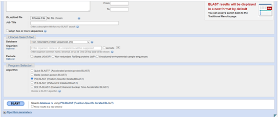
By default this is the standard protein BLAST, BLASTP. I want to use PSI-BLAST. To do this I scroll down the page a bit and find the radio buttons in the Program Selection section just above the blue BLAST button and be sure to select PSI-BLAST.
Image of the Standard Protein BLAST submission form (bottom).
Having done that I will now fill out the rest of the form to be able to do my PSI-BLAST. At the top of the form it says enter Query Sequence. This is the sequence that I want to know more about. This is my hypothetical protein sequence. There are several options for how to enter or give BLAST access to the sequence information. I am going to put in the FastA sequence by doing copy-paste from my Notepad file. With the sequence pasted into the large box at the top there is nothing else I need to in the first section of the form. The next part of the form says Choose Search Set. I am going to leave this as the default, which is to search the non-redundant protein sequences database. I’ve already done the Program Selection, having chosen PSI-BLAST. I can tick the box at the bottom to say I want the results shown in a new window. This can be useful if you want to run several searches because you can reset the form and have your results appear in new windows when they are complete. To run the search press the blue button that says BLAST.
Depending on the time of day and how busy the servers at NCBI are, it can take some time to run your PSI-BLAST search (or any BLAST search). This is why it can be useful to have your search results show in a new window. You can then have the form available for doing more investigations while you wait.
The results screen has several tabs where the results of your search will be displayed. For PSI-BLAST, additional iterations can be run, which is the purpose of PSI-BLAST. It will find more and more distantly related similar sequences to those that you take from the list to select for PSI-BLAST second and third iteration searches.
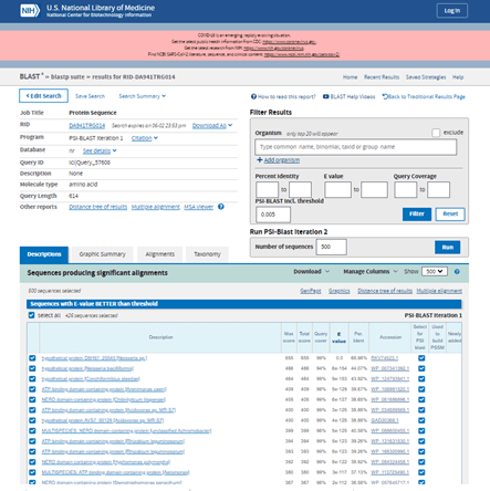
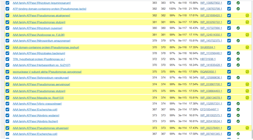
Image of PSI-BLAST results, Iteration 1.
For my results the top three hits are other hypothetical proteins but further down the list is an ATP-binding domain-containing protein and a NERD domain-containing protein. I am able to select or restrict the number of sequences or specific sequences to include in iteration 2 of the PSI-BLAST. I can do this using the blue tick boxes for individual sequences or by entering the number of sequences to include in the box under the Run PSI-BLAST Iteration 2 heading. I’m going to leave this at the default 500 sequences and press the blue Run button.
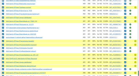
Scrolling down through the results of the second iteration the table shows with ticks in green circles those that were used to do the first iteration in one of the columns. Those that are newly added have a green tick in a new column and are highlighted in yellow. This makes it easy to identify newly discovered proteins that are similar to my original protein.
Image of PSI-BLAST results, Iteration 2, farther down the screen.
I have decided to try my luck and run a third iteration just to see what comes up. Some of the PSI-BLAST hits could be very dissimilar when we do repeated iterations, however we might also discover something interesting that could lead us to some insight. It is important that as scientists we critically assess the data in front of us. So once I collected the data, I’ll need to look at it and decide what contributions these results make to my understanding of the hypothetical protein.
At iteration three the new data is much further down the list and I can see that the similarity is much lower. The Query cover (the third column of numbers, expressed as a percentage) has gone from around 99% to around 68%. This means that less of the length of my protein is similar to these proteins. Also the Percent Identity is lower (the column of numbers before the hyperlink, expressed as a percentage) has gone very low, to the mid-teens. This means the proteins are not very similar. However, these proteins are all within a similar family to those previously recovered in iteration 2, which had higher coverage and a slightly higher Percent Identity score.
Image of PSI-BLAST results, Iteration 3, farther down the screen.
Therefore at the end of my PSI-BLAST research into my hypothetical protein of interest I have a few avenues for further investigation. My potential protein has similarity to sequences that contain ATP-binding domain-containing protein sequences and a NERD domain-containing protein sequences. In addition, it shares some limited homology with AAA family ATPases. Between the similarity to the ATP-binding domain-containing proteins and these, there might be some ATP dependent activity of my hypothetical protein, which I will need to investigate further.
I will now need to read about these domains and these types of proteins to be able to assess the outcome of my PSI-BLAST and decide what I’m going to do next with this information. I will also be sure to look at the data on the other tabs: Graphical Summary; Alignments; and Taxonomy, so see what more this view of the data can tell me. I might go back and re-run the PSI-BLAST and look at this detailed information at each iteration and possibly follow the links for specific proteins of interest to learn more.
Bacterial Genetics and Genomics book Discussion Topic: Chapter 20, question 14
This is the first time since I started this blog that I have been able to do it with a physical copy of the book at hand! It is so exciting to finally have tangible evidence of my hours of writing and to see the excellent finished product made possible through Patrick Lane’s talents bringing my pencil drawings to life in full-color illustrations and designing the cover, as well as the production team putting on the final touches.
It seems that most of the topics in the news and in academic circles on Twitter are in some way related to COVID-19. With that in mind, I have chosen to blog about azithromycin, which has been used in the treatment of some COVID-19 patients. Azithromycin is an antibiotic, which has antibacterial activity against some species of disease-causing bacteria. It is not used as an antibacterial against Pseudomonas aeruginosa, but azithromycin does have antibiofilm activity. Biofilms can be formed by some bacterial species like P. aeruginosa on natural and artificial surfaces and are a major health problem, due to their resistance to treatment. Biofilms are explored in Bacterial Genetics and Genomics in Chapters 5, 6, and 13.
To explore new research in the application of azithromycin for antibiofilm treatment of P. aeruginosa, I have selected a January 2020 paper that proposes antibiotic delivery directly to the biofilm location.
Lim DJ, Skinner D, Mclemore J, Rivers N, Elder JB, Allen M, Koch C, West J, Zhang S, Thompson HM, McCormick JP, Grayson JW, Cho DY, Woodworth BA. In-vitro evaluation of a ciprofloxacin and azithromycin sinus stent for Pseudomonas aeruginosa biofilms. Int Forum Allergy Rhinol. 2020 10(1):121-127. doi: 10.1002/alr.22475.
Rather than using a systemic antibiotic, a targeted delivery approach will mean that the antibiotic is at the concentration needed at the site of infection so that it can most effectively eliminate the bacteria and also possibly reducing side effects. In this case, the concern is P. aeruginosa chronic rhinosinusitis (sinus infection). Biofilms form in the sinuses and are very difficult to treat effectively using oral or IV antibiotics. Instead, these authors have recommended making a sinus stent that will deliver antibiotics directly to the biofilm. The ciprofloxacin-azithromycin sinus stent used in this study was constructed with two antibiotics, which both modulates the release of the drugs due to their different hydrophobic properties and also gives the stent two different antibacterials to combat the biofilms. Although we tend to study single species biofilms in the lab, those that occur in nature – and inside us – are often complex communities, so a multi-drug approach may be a good idea.
Coating the stents with both antibiotics prolonged the release of the ciprofloxacin, versus stents that were just coated with ciprofloxacin on its own. This is due to the hydrophobic nature of azithromycin, which was coated on the outside of the stents and meant that the ciprofloxacin wasn’t released in just one burst, as it was when there was no azithromycin.
In vitro, the stents with azithromycin and ciprofloxacin had good activity against P. aeruginosa biofilms. Interestingly, the authors note that they included azithromycin in the design of the stent only because of its hydrophobic properties, so that it would stop the burst release of the ciprofloxacin. They mention that it has positive anti-inflammatory benefits in treatment and that they will look at increasing concentrations of both antibiotics when moving to in vivo studies, but there is no mention of the antibiofilm activity of azithromycin against P. aeruginosa, which is known and used as a positive control for experiments investigating other antibiofilm drugs. This is another positive in favor of the decision of Lim et al. to use azithromycin as the hydrophobic outer drug for their sinus stent.
Skindersoe ME, Alhede M, Phipps R, Yang L, Jensen PO, Rasmussen TB, et al. Effects of antibiotics on quorum sensing in Pseudomonas aeruginosa. Antimicrob Agents Chemother. 2008 52:3648–3663. doi: 10.1128/AAC.01230-07.
Seleem NM, Abd El Latif HK, Shaldam MA, El-Ganiny A. Drugs with new lease of life as quorum sensing inhibitors: for combating MDR Acinetobacter baumannii infections. Eur J Clin Microbiol Infect Dis. 2020. doi: 10.1007/s10096-020-03882-z.
Repurposing of antibiotics and thinking about them in new ways in which we can use them to fight infections are important points for discussion. Understanding bacterial genetics and genomics gives us insights into biofilms and antimicrobial susceptibilities that can drive ongoing and future research.
Bacterial Genetics and Genomics book Discussion Topic: Chapter 1, question 13
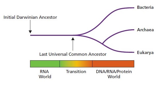
In honor of today, the day my book is released to the world, I have decided to blog on the topic of the very first Discussion Topic in the book. This relates to the Last Universal Common Ancestor (LUCA) before what we recognize now as bacteria, archaea, and eukaryotes and the common features we still see in them. I came across this paper (https://www.jbc.org/content/295/8/2313) by Michael W. Gray and Venkat Gopalan in the Journal of Biological Chemistry called ‘Piece by piece: Building a ribozyme’. It focuses on ribosomes, which are central to translation, and RNase P, which is part of tRNA processing. Both ribosomes and RNase P were present in the LUCA.
Ribosomes and RNase P have in common that they have within them ribozyme activity and this catalytic RNA action is fundamental to their function. Ribozymes are, as described in Bacterial Genetics and Genomics, an RNA with enzymatic activity.
In this paper, the story of how RNAs evolved is built, starting from what is believed to be the oldest of the activities within the ribosome, its peptidyl transferase center. The model discussed in this review looks at how fragments of RNA with different functional domains would have accumulated over evolutionary time to become the rRNA sequences that we see now within the ribosomes. Likewise, for RNase P, which is involved in tRNA 5ˈ maturation, the model discussed proposes the progressive evolutionary addition of functional domains. For both models, the authors draw on the literature and years of experimental work and theoretical work to describe how these processes are likely to have evolved.
In summary, Gray and Gopalan show how the long non-coding RNAs like those present in the large subunit rRNAs and in the RNA subunit of RNase P have evolved from smaller RNAs. The origins of these sequences were, over time, “stitched together” to become what we see in genome sequences today. This both explains the common origin of these ribozymes that are shared amongst the bacteria, archaea, and eukaryotes and also provides for the diversity in the lineages, including the 16S, 23S, and 5S rRNAs in bacteria and archaea compared to the 18S, 28S, 5S, and 5.8S rRNAs in eukaryotes.
Bacterial Genetics and Genomics book Discussion Topic: Chapter 12, question 15
I saw a Tweet about a paper on pangenome analysis and decided to read it. It is on bioRxiv, the preprint server for biology (https://www.biorxiv.org/). The papers here aren’t peer reviewed, like to you would find in typical journals, so when you read something here, it relies on your own critical analysis and assessment of what is being presented by the authors even more than usual. No reviewers or editors have looked at these papers. They haven’t already been through revisions based on reviewers comments and haven’t then been changed before an editor will release them for general reading. They are put on the server as the authors wrote them and this is done because the authors feel they have an important message that needs to be out there. It also is a forum for the authors to get feedback from a wider pool of scientists than just 2 to 4 reviewers and an editor on their manuscript, which they can use to revise it and then perhaps submit it to a peer-reviewed journal.
Looking at this pangenome paper, I recognized some of the authors named and immediately knew that not only did I want to read it because the topic was interesting, but I knew these authors as past collaborators and contributors to the field of bacterial genomics, so I wanted to read what they had to say. I was delighted to see right from the abstract, agreements with points made in my book about some of the pitfalls with automated annotations. Even better was claim that they have devised a system to overcome some of those problems with a graph based pangenome clustering tool called Panaroo.
As more and more bacterial genomes are being generated, more and more sequence data is being annotated. Since this uses automated annotation systems and is often infrequently manually curated on a gene-by-gene basis by someone with intimate knowledge of the genomics of the bacterial species (who has time to do that for a thousand genomes?), there are inevitable errors. Errors in one genome are replicated in others and so on. These errors impact studies that look at pangenomes, which start by identifying all of the orthologous CDSs. Also problematic are fragmented assemblies of the genomic data, mis-assemblies (where the data is put together in the wrong order), and contamination (where sequence data from another source is present in the reported data – something that happens far more than we like to admit!). If a core gene is fragmented, so that half of it is present in one contig and half of it is present in another contig (see Bacterial Genetics and Genomics Figure 17.15), then that core gene isn’t identified and can’t be included in the pangenome analysis and will be reported as absent in that isolate, which might mean it is removed from the core genes list. In the case of the gene in the Figure 17.15 example, that gene is dnaA; it is core and important for bacteria. So, there is a problem with fragmented genome sequence data, as well as errors in annotations.
Panaroo shares information between genomes to improve annotation calls, which improves the clustering of the orthologues and paralogues. The tools in Panaroo empower the researchers and have been tested against genome sequence data and compared to the results from other pangenome analysis tools. Simulated genome sequence data sets were used that included contamination and genome fragmentation. One was for Mycobacterium tuberculosis, which is a highly conserved species that has little variation in its genome. The other data set was made of Klebsiella pneumoniae genome sequence data, which is highly diverse. Panaroo was superior in its analysis of both datasets compared to other pangenome tools in identifying the core and accessory genomes. In addition, there are tools within Panaroo that allowed the researchers to identify 9 samples within the K. pneumoniae dataset that were outliers during the quality control stage, before pangenome analysis. Other tools within Panaroo allow users to conduct pangenome genome wide association studies (pan-GWAS) to find genetic features from a collection of genome sequences that might be associated with phenotypes and tools that investigate pangenome evolution. This led to some new discoveries in a few species discussed in the paper. These are genome sequence datasets that are not simulated test data for Panaroo, but actual genomic data, where after having tested Panaroo on the M. tuberculosis and K. pneumoniae datasets, they then tried it out on some other species to see what they would find. The results are quite interesting and they found some novel and in some cases unexpected features.
Bacterial Genetics and Genomics book Discussion Topic: Chapter 11, question 14.
Last week I attended the Festival of Genomics in London. These are excellent events, run by Front Line Genomics and due to the support of many sponsors, they are free to attend. Going to the Festival of Genomics is an excellent opportunity to hear some outstanding talks about current research in the field, speak to vendors supporting genomic technologies, and network.
One of the most exciting things I saw was the Oxford Nanopore sequencer that fits in the palm of your hand. As described in my book, Bacterial Genetics and Genomics, nanopore sequencing can directly read the sequence of the DNA strand. This new equipment is the MinION Mk1C and combines the previous MinION, which was about the size of a big USB stick, and the computing of a standard laptop needed to run the MinION. The MinION Mk1C eliminates the need for a laptop, which means the whole sequencer can easily go in a small bag or the pocket of your cargo pants trousers. When doing field work, such as traveling to areas of outbreaks and doing real-time epidemiology, reducing the amount of extra equipment is important.
Below is a Tweet I sent out at the Festival of Genomics, which includes a video of the MinION Mk1C. As you watch the video, along the bottom of the device is the flowcell, where the sequencing is happening. The screen is showing the status of the sequencing in real-time. When the video pans to the left, you will see the standard MinION device, which holds one flowcell and via USB plugs into a laptop to run. All the computing power and software needed for sequencing and analysis is available on this one device.
In speaking to the Oxford Nanopore representatives at the Festival of Genomics, I was told that they have also miniaturized and simplified the sample preparation process with the VolTRAX system, which is about the size of the MinION and USB powered. Of course, all of the sequencing and sample preparation will require electricity, but I was told that if there aren’t any outlets available in the field location, the devices will run on powerpacks. So, truly portable, small sequencing is in the palm of our hands.
Although the MinION Mk1C has only recently become available to purchase, the technology behind it has been in the MinION and other Oxford Nanopore systems for a few years now. There are many papers that have used this technology to address bacterial epidemiology, which is Discussion Topic question 14 for Chapter 11. In addition to my general tips distributed with the book, for this question, if you are interested in application of nanopore sequencing, go to the Oxford Nanopore web site and check out their Resource Centre with its listing of papers citing their technology. I particularly like this one by Leah W. Roberts et al. from Nature Communications 2020 describing use of three types of whole genome sequencing methods to investigate an outbreak of carbapenemase-producing Enterobacter hormaechei. It is interesting to see both what they found in the analysis of the hospital outbreak and also how they used Illumina, Pacific Biosciences, and Oxford Nanopore data together to achieve their goals.
As my book went off to press, sequencing was in the news as it is being applied to the coronavirus outbreak. New and exciting events like this are not captured in the book, but can be included in a blog.
Yes, viruses like the coronavirus are outside of the scope of my book – viruses are not bacteria, however the application of sequencing technology to epidemiology and outbreaks is absolutely covered in the book and students who read the book will be able to apply what they know from the bacterial examples to this viral disease. In the same way, students wanting to go on to study higher organisms will find that the grounding they get from the concepts in Bacterial Genetics and Genomics will have wider applications in humans, animals, plants, etc. Much of what we know now in genetics and genomics in general started in bacteria and interesting discoveries made in bacteria (like CRISPR) keep getting applied elsewhere.
Bacterial genetics and genomics is a rapidly advancing field. I have written the book to be as flexibly future proof as possible, by including some examples of recent advances, but also encouraging you as the reader to explore more. In this blog, I can continue to keep the discussion current and help guide you in finding some interesting topics for discussion in class, with friends, or on-line.